Moneyball Lacrosse
I drew inspiration for this project from a variety sources. First, from the movie Moneyball based off the book by Michael Lewis. Then from Analytics Edge, a course offered by edX and MIT, where we went through how the Oakland A’s used statistics to gain a competitive edge over opponents.
After the course, I thought why not do it for Lacrosse, a sport that I have played since I was five. When researching whether or not such an analysis had been done before, I stumbled upon an insightful article written in 2011 by Michael Mauboussin, which has unfortunately become a dead link. I borrowed insights that he described in the article in addition to exploring different metrics.
Data
I scraped the data from the http://stats.ncaa.org/. I did this mainly with the Selenium package. Selenium is a great tool that allows you to write scripts that can do a variety of different actions on a website (i.e. clicking). This is really important when dealing with interactive websites like the NCAA’s. To see how I extracted the data for this project, check out the scrape.py.
Attributes of the extracted data:
  Seasons: 2011 - 2019
  Rows, Cols: (602, 11)
  Fields: Team, Conference, Year, Games, Won, Lost, WinPct, Goals, GPG,
          Goals Allowed, GAPG, Playoffs
Pythagorean Expectation
According to the Wikipedia page, “the Pythagorean expectation is a sports analytics formula devised by Bill James to estimate the percentage of games a baseball team ‘should’ have won based on the number of runs they scored and allowed. Comparing a team’s actual and Pythagorean winning percentage can be used to make predictions and evaluate which teams are over-performing and under-performing. The name comes from the formula’s resemblance to the Pythagorean theorem.”
I have adapted this formula slightly for lacrosse by using the goals scored and allowed:
def calculate_pythagorean_expectation(df, exp=2):
    return 1 / 1 + (df["Goals"] / df["Goals Allowed"])**exp
After experimenting with many exp values, I found that the optimal value for predicting win percentage was 1.23. It is common practice to adapt this value according to the sport domain. For instance, statisticians who analyze the NBA use a value of 13.91 while their counterparts in the NFL use 2.37.
Preprocess data
So once we have an expectation formula, we can calculate the expected win percentage and wins for a given year:
df.loc[:, "ExpectWinPct"] = calculate_pythagorean_expectation(df, exp=1.23)
df.loc[:, "ExpectWon"] = df["Games"] * df["ExpectWinPct"]
Train model
We will use the ExpectWon feature and data from 2011-2018 to train a simple ordinary least squares (ols) model using the statsmodels package. Once the model is trained, will will be able to make predictions for the 2019 season.
import statsmodels.api as sm

X, y = train.ExpectWon, train.Won
model = sm.OLS(y, X).fit()
For those who are not familiar with an OLS model, it basically fits a straight line to the data where the errors are the smallest. You can see the model plotted on the training data below:
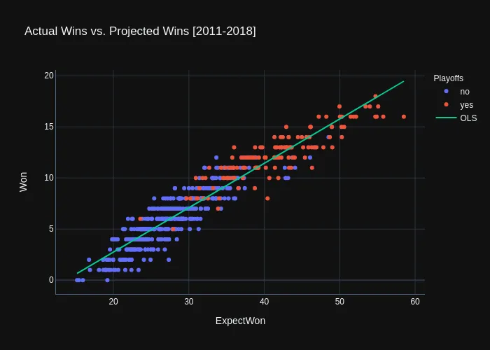
As you can see, the model does a decent job at predicting wins, but we can even get a more detailed view of its performance by looking at the model.summary():
                      OLS Regression Results
==============================================================================
   Adj. R-squared:                  0.891**
==============================================================================
                 coef    std err          t      P>|t|      [0.025      0.975]
------------------------------------------------------------------------------
const         -5.9420      0.214    -27.796      0.000      -6.362      -5.522
ExpectWon      0.4344      0.007     65.505      0.000*      0.421       0.447
==============================================================================
First thing to point out here is that the ExpectWon is indeed statistically significant (P>|t| < 0.05)* in predicting the actual wins. Another important metric is the adjusted R-squared which has a value of 0.891**. This means that about 89.1% of the variance in the data can be explained by the ExpectWon feature.
Predict Wins
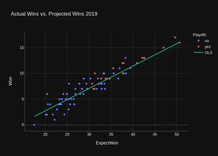
Now that we have a trained model, let’s make predictions for the 2019 season:
    year             team  won       pred
0   2019        Air Force   10  10.504494
1   2019           Albany    5   5.541597
2   2019  Army West Point   13  12.577771
3   2019       Bellarmine    3   3.898540
4   2019       Binghamton    2   2.887904
..   ...              ...  ...        ...
68  2019          Vermont    8   8.341417
69  2019        Villanova    8   6.819309
70  2019         Virginia   17  15.609287
71  2019           Wagner    2   3.487773
72  2019             Yale   15  14.474503
[73 rows x 4 columns]
Here is how it looks graphically:
What Leads to a Win
This shows only the big picture of what makes a team succesful, but it does not tell us what leads a team to win games. Thus we need to individually look at what contributes to a good offense (efficient possessions that end in goals) and good defense (possessions that lead to turnovers or saves).
Predicting the number of wins that a team will win is great in all, but not every team plays the same amount of games. So from now on we are going to concentrate on the variables that effect WinPct.
Offense vs. Defense
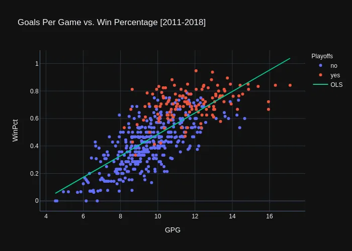
We now know that a good offense and defense contributed to a successful season, but which side of the field is more important? To determine this we are going to train to separate OLS models and compare whether Goals per Game or Goals Against per game is more influential on WinPct.
Offense
                            OLS Regression Results
==============================================================================
  Adj. R-squared:                  0.558**
==============================================================================
                 coef    std err          t      P>|t|      [0.025      0.975]
------------------------------------------------------------------------------
const         -0.2962      0.031     -9.587      0.000      -0.357      -0.235
GPG            0.0780***   0.003     25.830      0.000*      0.072       0.084
==============================================================================
It appears from the OLS results that GPG is indeed significant* and explains roughly 55.8%** of the variance in the data. You can interpret the GPG coefficient as an increase in 1 goal per game results in a 7.8%*** increase in WinPct.
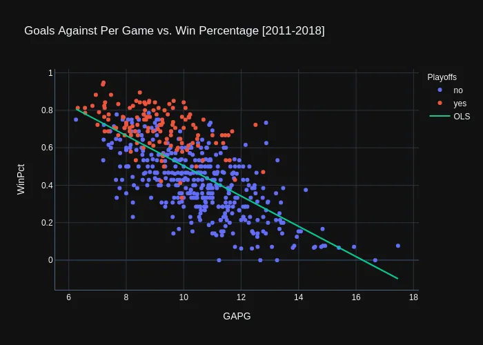
Defense
                            OLS Regression Results
==============================================================================
  Adj. R-squared:                  0.477**
==============================================================================
                 coef    std err          t      P>|t|      [0.025      0.975]
------------------------------------------------------------------------------
const          1.3108      0.038     34.493      0.000       1.236       1.385
GAPG          -0.0807***   0.004    -21.988      0.000*     -0.088      -0.074
==============================================================================
It appears from the OLS results that GAPG is also significant* and explains roughly 47.7%** of the variance in the data. You can interpret the GAPG coefficient as an increase in 1 goal against per game results in a 8.1%*** decrease for a team’s WinPct.
Optimize Offense
Although offense and defense are both predictive in determining WinPct, offense is slightly more important (as I was hoping). So we will concentrate on how to maximize GPG, which should thus improve WinPct.
Although there a many factors that influence offense, I’ve narrowed it down to three factors: shooting, groundballs, and faceoffs. I have devised three simple hypotheses:
- Shooting -> more shots (on goal) => more goals
- Groundballs -> more groundballs => more goals
- Faceoff % -> higher percentage => more goals
Let’s see if the saying “ground balls win games” holds true. [To be continued]